第一章-学习之前的认知
影响股价的因素
1、公司自身因素
2、心理因素
3、行业因素
4、经济因素
5、市场因素
6、政治因素
金融量化投资
量化投资的优势
1、避免主观情绪,人性弱点和认知偏差,选择更加客观
2、能同时包括多角度的观察和多层次的模型
3、及时跟踪市场变化,不断发现新的统计模型,寻找交易机会
4、在决定投资策略后,能通过回测验证其效果
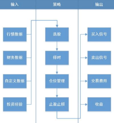
量化策略
  通过一套固定的逻辑来分析、判断和决策,自动地进行股票交易
策略的周期
  实现想法、学习知识
  实现策略:python
  检验策略:回测、模拟交易
  实盘交易
  优化策略,放弃策略
第二章-科学计算基础包---numpy
量化投资和python
为什么选择python呢?
其他选择:excel、SAS/SPSS(统计软件,无编程)、R(功能太单一,制作数据分析)

量化投资实际上就是分析数据从而做出决策的过程
python数据处理相关模块
    1、NumPy:数组批量计算
    2、pandas:灵活的表计算
    3、Matplotlib:数据可视化
怎么使用python进行量化投资
自己编写
    NumPy + pandas + Matplotlib....
在线平台
    聚宽、优矿、米筐、Quantopian....
开源框架
    RQAlpha、QUANTAXIS....
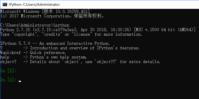
IPython的使用
pip3 install ipthon
也可以直接安装anacoda ,集成了ipython、NumPy pandas Matplotlib 等许多python的常用模块和框架
与python解释器的使用方法一致
TAB键自动完成
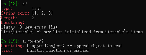
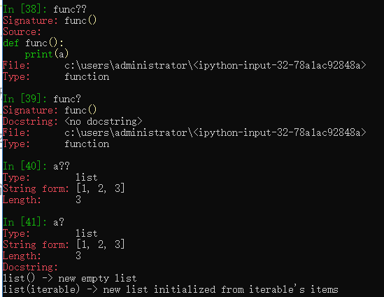
?内省、查看具体信息
?进行模糊匹配,命名空间搜索
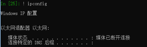
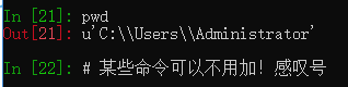
!执行系统命令
某些命令不用加也能执行
??两个问号
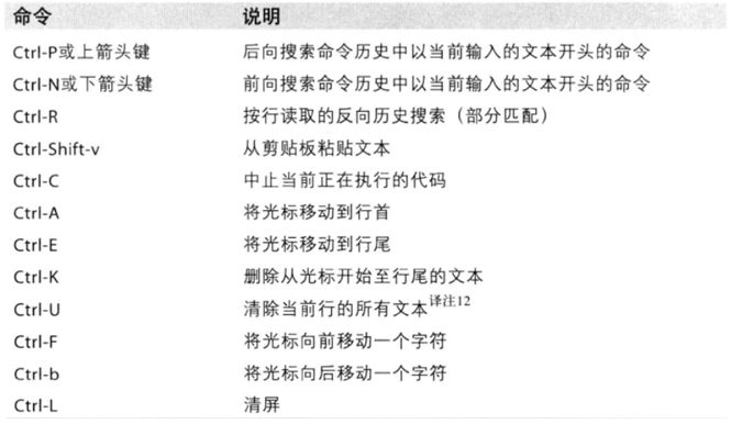
快捷键
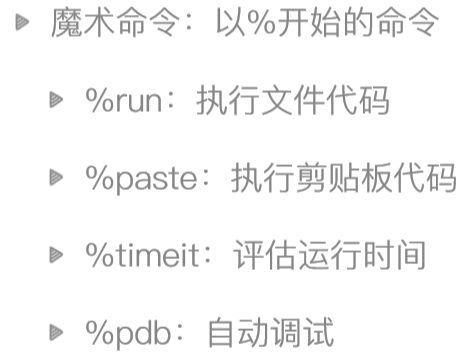
IPython的魔术命令
%timeit 很费事,他要跑很多次
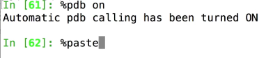
%paste 执行剪切板中的python代码
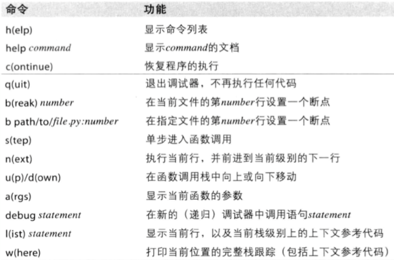
%pdb 在异常发生后自动进入调试模式,使用on
然后就可以使用pdb相关的命令,进行调试状态
p命令最常用,打印的意思
%魔术命令
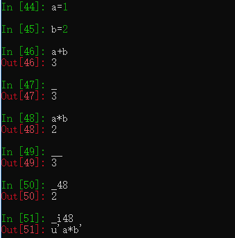
命令的历史可以使用上下方向键,或者%hist查看命令历史
_ 表示上一次的输出
__ 表示上两个命令
_48 第多少的结果
_i48 第多少行的结果的字符串形式
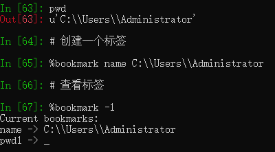
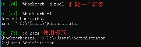
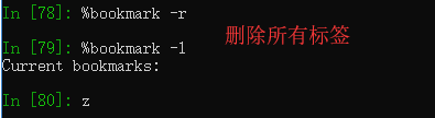
%bookmark 目录标签系统
IPython Notebook-Jupyter的初识
安装jupyter
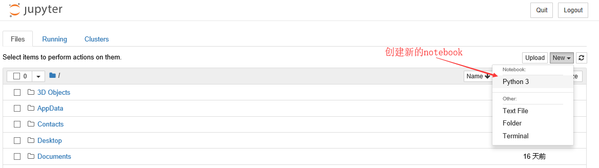
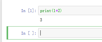
使用notebook
进入了jupyter的web界面
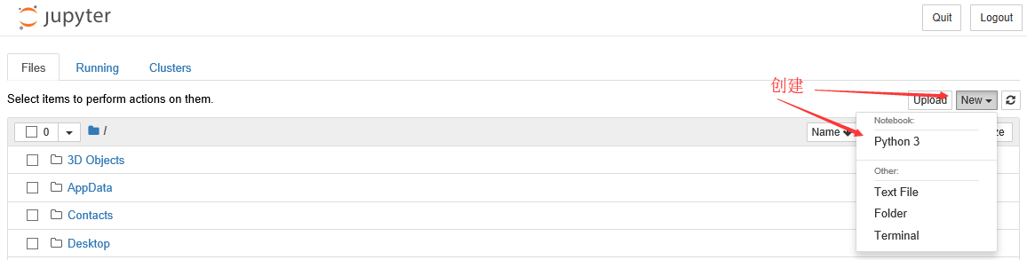
创建新的notebook
出现一个小问题:编写的代码不能运行且前面的提示符In
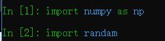
查看命令行,出现错误提示
将软件降级安装后,解决问题
可以用notebook写博客,支持makedown,而且他可以将页面直接输出成很多文本形式
正戏-Numpy模块
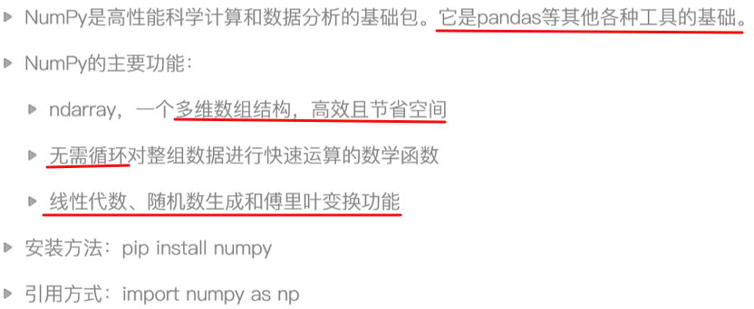
Numpy简介
实例展示为什么要使用numpy
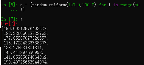
例子:已知若干家跨国公司的市值,将其换算成人民币
普通的函数方法
1、将公司市值存储成列表或者其他格式
2、创建变量,存储汇率
2、遍历列表
3、做乘法运算,放入新的列表
用numpy
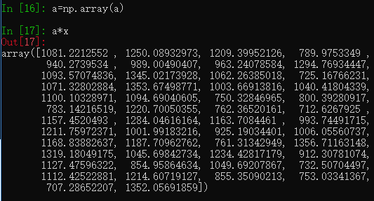
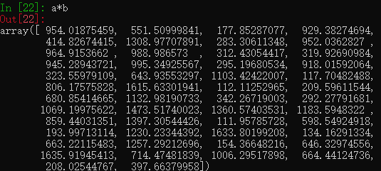
例子2:已知每件商品的价格和每件商品的数量,计算总金额
还是用a作为价格,再创建一个数组作为每件商品的数量
计算每件商品的价格
计算总金额
ndarray-多维数组对象
ndarray-常用属性
In [26]: a.ndim
Out[26]: 1
In [27]: a.size
Out[27]: 50
In [28]: a.shape
Out[28]: (50,)
-----------------------------
In [30]: b = np.array([[1,2,3,],[4,5,6]])
In [31]: b.ndim
Out[31]: 2
In [32]: b.size
Out[32]: 6
In [33]: b.shape
Out[33]: (2, 3)
-----------------------------
三维-第三个维度相当于笔记本的每一页,翻个页就到另一面
In [35]: c = np.array([[[1,2,3,],[4,5,6]],[[1,2,3],[1,2,3]]])

In [36]: c
Out[36]:
array([[[1, 2, 3],
        [4, 5, 6]],

       [[1, 2, 3],
        [1, 2, 3]]])
In [37]: c.shape
Out[37]: (2, 2, 3)
------------------------------------
数组的转置
In [39]: c = c.T

In [40]: c
Out[40]:
array([[[1, 1],
        [4, 1]],

       [[2, 2],
        [5, 2]],

       [[3, 3],
        [6, 3]]])

In [41]: c = c.T

In [42]: c
Out[42]:
array([[[1, 2, 3],
        [4, 5, 6]],

       [[1, 2, 3],
        [1, 2, 3]]])
ndarray-数据类型
查看数据类型
In [24]: a.dtype
Out[24]: dtype('float64')
我们使用的巨大部分都是数字类型,它本身就是用来做计算的
64位数的长度是多少(2**63-1)
In [25]: 2**64-1
Out[25]: 18446744073709551615
numpy-array的创建
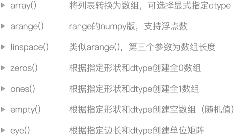
In [1]: # 可以这样创建一个10位全是0的数组
In [2]: import numpy as np
In [3]: a = np.array([0]*10)
In [4]: a
Out[4]: array([0, 0, 0, 0, 0, 0, 0, 0, 0, 0])

In [5]: # 也可以用zeros创建
In [6]: b = np.zeros(10)
In [7]: b
Out[7]: array([0., 0., 0., 0., 0., 0., 0., 0., 0., 0.])

In [8]: # 可以看见都是0.,说明他是一个浮点数,来看一下类型
In [9]: b.dtype
Out[9]: dtype('float64')

In [10]: # 创建的时候指定类型,不使用默认的,直接用int
In [11]: c = np.zeros(10,dtype='int')
In [12]: c
Out[12]: array([0, 0, 0, 0, 0, 0, 0, 0, 0, 0])
In [13]: c.dtype
Out[13]: dtype('int32')

In [14]: # 创建全是1的数组
In [15]: d = np.ones(10)
In [16]: d
Out[16]: array([1., 1., 1., 1., 1., 1., 1., 1., 1., 1.])

In [17]: # 看一下empty的用法,创建空数组,里面放的都是随机数
In [18]: e = np.empty(50)
In [19]: e
Out[19]:
array([1.23004319e-311, 1.23004150e-311, 2.95806213e-311, 1.26927730e-277,
       5.54041819e+228, 2.84855906e-311, 5.97288716e-299, 3.28487474e-311,
       9.43293441e-314, 2.26784710e-308, 1.23004306e-311, 1.23002517e-311,
       3.38460664e+125, 6.69053866e+151, 6.56693077e-085, 1.03564308e-308,
       1.33360293e+241, 1.71632673e+243, 5.96115807e+228, 1.71011791e+214,
       5.67517369e-311, 1.00562508e-248, 2.85308965e-313, 2.14793507e-308,
       1.38760675e+219, 2.92135768e+209, 2.21211602e+214, 2.28723653e-308,
       6.96983359e+228, 1.33360298e+241, 2.11280666e+161, 1.29883065e+219,
       1.11074825e-310, 1.46972270e-200, 4.97508544e-313, 4.65203811e+151,
       4.66820502e+180, 5.61168418e-313, 3.81674046e-308, 1.33360303e+241,
       1.54523733e-310, 5.03961303e-266, 3.99046880e-008, 2.08868046e-310,
       2.53185169e-212, 7.44726967e-251, 1.39069238e-309, 2.75926410e-306,
       4.90398331e-307, 5.23951796e+202])
In [20]: #  这些随机值是,之前内存的残存值。这个empty有什么用呢?
In [21]: #  为了之后给里面赋值,因为它相对于zeros和ones创建的时候少了1个步骤,会更快一点

In [22]: # arange可以指定步长为小数,pyton中是不可以的
In [24]: f = np.arange(1,10,0.3)
In [25]: f
Out[25]:
array([1. , 1.3, 1.6, 1.9, 2.2, 2.5, 2.8, 3.1, 3.4, 3.7, 4. , 4.3, 4.6,
       4.9, 5.2, 5.5, 5.8, 6.1, 6.4, 6.7, 7. , 7.3, 7.6, 7.9, 8.2, 8.5,
       8.8, 9.1, 9.4, 9.7])

In [26]: # linspace线性空间,和arange非常相,但是完全不一样,把指定的范围数字分成间隔相同的份数,最后一个参数是数组的长度,即份数
In [31]: k = np.linspace(0,5,10)  或者是  np.linespace(0,5,num=10)
In [32]: k  #并且linspace不像arange不包含最后一个数,它是包含最后一个数的,可以在最后看见5
Out[32]:
array([0.        , 0.55555556, 1.11111111, 1.66666667, 2.22222222,
       2.77777778, 3.33333333, 3.88888889, 4.44444444, 5.        ])
In [27]: g = np.linspace(1,100,100)
In [28]: g
Out[28]:
array([  1.,   2.,   3.,   4.,   5.,   6.,   7.,   8.,   9.,  10.,  11.,
        12.,  13.,  14.,  15.,  16.,  17.,  18.,  19.,  20.,  21.,  22.,
        23.,  24.,  25.,  26.,  27.,  28.,  29.,  30.,  31.,  32.,  33.,
        34.,  35.,  36.,  37.,  38.,  39.,  40.,  41.,  42.,  43.,  44.,
        45.,  46.,  47.,  48.,  49.,  50.,  51.,  52.,  53.,  54.,  55.,
        56.,  57.,  58.,  59.,  60.,  61.,  62.,  63.,  64.,  65.,  66.,
        67.,  68.,  69.,  70.,  71.,  72.,  73.,  74.,  75.,  76.,  77.,
        78.,  79.,  80.,  81.,  82.,  83.,  84.,  85.,  86.,  87.,  88.,
        89.,  90.,  91.,  92.,  93.,  94.,  95.,  96.,  97.,  98.,  99.,
       100.])

In [33]: #eye 生成单位矩阵,对角线上都是1,不做线性代数,基本不会遇到
In [37]: w = np.eye(5)
In [38]: w
Out[38]:
array([[1., 0., 0., 0., 0.],
       [0., 1., 0., 0., 0.],
       [0., 0., 1., 0., 0.],
       [0., 0., 0., 1., 0.],
       [0., 0., 0., 0., 1.]])
ndarray-批量运算
比较运算最后得到的是布尔值
如何快速生成一个二维数组
In [39]: np.arange(15).reshape((3,5))
Out[39]:
array([[ 0,  1,  2,  3,  4],
       [ 5,  6,  7,  8,  9],
       [10, 11, 12, 13, 14]])
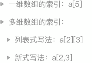
ndarray-索引
array([[ 0,  1,  2,  3,  4],
       [ 5,  6,  7,  8,  9],
       [10, 11, 12, 13, 14]])

In [40]: a = np.arange(15).reshape((3,5))

In [41]: a[2,2]
Out[41]: 12
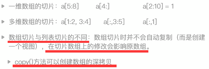
adarray-切片
也是前包后不包
In [46]: f
Out[46]:
array([1. , 1.3, 1.6, 1.9, 2.2, 2.5, 2.8, 3.1, 3.4, 3.7, 4. , 4.3, 4.6,
       4.9, 5.2, 5.5, 5.8, 6.1, 6.4, 6.7, 7. , 7.3, 7.6, 7.9, 8.2, 8.5,
       8.8, 9.1, 9.4, 9.7])

In [48]: f[1:3]
Out[48]: array([1.3, 1.6])
但是数组切片,为了省空间,在切片的时候只是浅拷贝
如果要不影响原数组,切片的时候使用copy
In [55]: b = f[0:5]

In [56]: b
Out[56]: array([1. , 1.3, 1.6, 1.9, 2.2])

In [57]: b[0] = 5

In [58]: b
Out[58]: array([5. , 1.3, 1.6, 1.9, 2.2])

In [59]: f
Out[59]:
array([5. , 1.3, 1.6, 1.9, 2.2, 2.5, 2.8, 3.1, 3.4, 3.7, 4. , 4.3, 4.6,
       4.9, 5.2, 5.5, 5.8, 6.1, 6.4, 6.7, 7. , 7.3, 7.6, 7.9, 8.2, 8.5,
       8.8, 9.1, 9.4, 9.7])
使用copy
b = f[0:5].copy()
多行切片
In [49]: a
Out[49]:
array([[ 0,  1,  2,  3,  4],
       [ 5,  6,  7,  8,  9],
       [10, 11, 12, 13, 14]])
In [50]: # 多行切片,可以看做是[切行,切列]
In [54]: a[0:2,0:2]
Out[54]:
array([[0, 1],
       [5, 6]])
ndarray-布尔型索引
需求:选出列表中大于5的数
In [60]: import random
# 用列表的filter方法
In [61]: a = [random.randint(0,10) for i in range(20)]
In [62]: a
Out[62]: [1, 2, 1, 6, 1, 8, 6, 7, 3, 0, 6, 8, 2, 6, 0, 1, 4, 10, 0, 3]
In [63]: list(filter(lambda x:x>5, a))
Out[63]: [6, 8, 6, 7, 6, 8, 6, 10]
# 用数组的布尔值索引
In [64]: a = np.array(a)
In [65]: a[a>5]
Out[65]: array([ 6,  8,  6,  7,  6,  8,  6, 10])

In [66]: # 布尔型索引的原理
In [67]: # 第一步 a>5
In [68]: a>5
Out[68]:
array([False, False, False,  True, False,  True,  True,  True, False,
       False,  True,  True, False,  True, False, False, False,  True,
       False, False])

In [69]: # 第二步,返回每一位置为ture的位置的值
In [70]: b = np.array([1,2,3])
In [71]: c = np.array([True,False,True])
In [72]: b[c]
Out[72]: array([1, 3])
需求2:选出数组中大于5的偶数
题外:and 和 & 有什么区别?
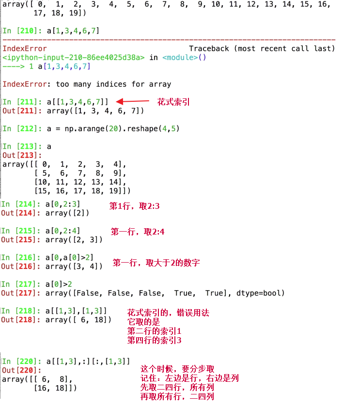
ndarray-花式索引
注意:多维数组中,花式索引和花式索引不能出现在,逗号的两边
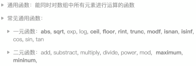
Numpy-通用函数
abs-批量求绝对值
In [2]: a = np.arange(-5,5)
In [3]: a
Out[3]: array([-5, -4, -3, -2, -1,  0,  1,  2,  3,  4])
# 直接用abs也可以
In [4]: abs(a)
Out[4]: array([5, 4, 3, 2, 1, 0, 1, 2, 3, 4])
# 严谨的用法是np.abs
In [5]: np.abs(a)
Out[5]: array([5, 4, 3, 2, 1, 0, 1, 2, 3, 4])
aqrt-开方
# 直接使用会报错,没有这个sqrt,找不到
In [7]: sqrt(a)
---------------------------------------------------------------------------
NameError                                 Traceback (most recent call last)
<ipython-input-7-55c08d4e5fa4> in <module>()
----> 1 sqrt(a)

NameError: name 'sqrt' is not defined
# math模块下有sqrt
In [8]: import math
# 报错,sqrt一次只能处理一个值
In [11]: math.sqrt(a)
---------------------------------------------------------------------------
TypeError                                 Traceback (most recent call last)
<ipython-input-11-c85d302be686> in <module>()
----> 1 math.sqrt(a)

TypeError: only size-1 arrays can be converted to Python scalars
# 使用np.sqrt ,因为负数不能求开方
In [10]: np.sqrt(a)
F:\Python36\Scripts\ipython3:1: RuntimeWarning: invalid value encountered in sqrt
Out[10]:
array([       nan,        nan,        nan,        nan,        nan,
       0.        , 1.        , 1.41421356, 1.73205081, 2.        ])
把一个小数变成整数-取整和保留小数位
In [12]: a = 1.6
# 这种取整,叫做向0取整
In [13]: int(a)
Out[13]: 1
# 这种叫做四舍五入
In [14]: round(a)
Out[14]: 2
# 向上取整-ceil
In [15]: math.ceil(a)
Out[15]: 2
# 向下取整-floor
In [16]: math.floor(a)
Out[16]: 1
# 使用np
In [18]: a
Out[18]: array([-5.5, -4.5, -3.5, -2.5, -1.5, -0.5,  0.5,  1.5,  2.5,  3.5,  4.5])
# 向下取整
In [19]: np.floor(a)
Out[19]: array([-6., -5., -4., -3., -2., -1.,  0.,  1.,  2.,  3.,  4.])
# 向上取整
In [22]: np.ceil(a)
Out[22]: array([-5., -4., -3., -2., -1., -0.,  1.,  2.,  3.,  4.,  5.])
# 四舍五入
In [23]: np.round(a)
Out[23]: array([-6., -4., -4., -2., -2., -0.,  0.,  2.,  2.,  4.,  4.])
# rint和round是一样的
In [20]: np.rint(a)
Out[20]: array([-6., -4., -4., -2., -2., -0.,  0.,  2.,  2.,  4.,  4.])
# 向0取整
In [21]: np.trunc(a)
Out[21]: array([-5., -4., -3., -2., -1., -0.,  0.,  1.,  2.,  3.,  4.])
注:这里的round用的是"四舍六入五成双,奇进偶不进"的方法。对于大量的计算而言,比普通的四舍五入要更科学
modf-把小数和整数部分分开获取
In [26]: np.modf(a)
Out[26]:
(array([-0.5, -0.5, -0.5, -0.5, -0.5, -0.5,  0.5,  0.5,  0.5,  0.5,  0.5]),
 array([-5., -4., -3., -2., -1., -0.,  0.,  1.,  2.,  3.,  4.]))

In [27]: x,y = _

In [28]: x
Out[28]: array([-0.5, -0.5, -0.5, -0.5, -0.5, -0.5,  0.5,  0.5,  0.5,  0.5,  0.5])

In [29]: y
Out[29]: array([-5., -4., -3., -2., -1., -0.,  0.,  1.,  2.,  3.,  4.])
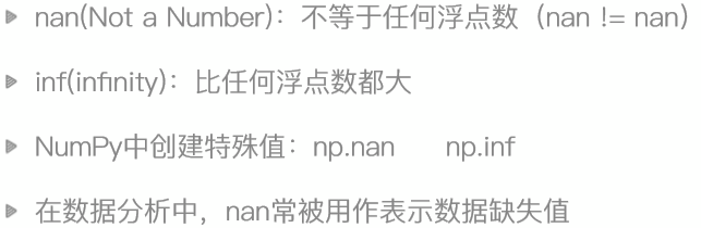
isnan和isinf-浮点数特殊值的判定
In [31]: a = np.ones(5)

In [32]: a
Out[32]: array([1., 1., 1., 1., 1.])

In [33]: a[1] = 0

In [34]: a
Out[34]: array([1., 0., 1., 1., 1.])

In [36]: b = a/a
F:\Python36\Scripts\ipython3:1: RuntimeWarning: invalid value encountered in true_divide

In [37]: a
Out[37]: array([1., 0., 1., 1., 1.])

In [38]: b
Out[38]: array([ 1., nan,  1.,  1.,  1.])

In [39]: 1 in b
Out[39]: True
# 这样判断对nan是无用的
In [40]: np.nan in b
Out[40]: False
# isnan的作用
In [41]: np.isnan(b)
Out[41]: array([False,  True, False, False, False])
isnan用来取值
In [42]: b[np.isnan(b)]
Out[42]: array([nan])

In [43]: b[~np.isnan(b)]
Out[43]: array([1., 1., 1., 1.])
inf-比任何数都大
In [44]: np.inf > 1000000000000000000000000000000
Out[44]: True

In [45]: float('inf') > 1000000000000000000000000000000000
Out[45]: True
inf和isinf的使用
In [46]: a = np.array([3,4,5,6,7])
In [47]: b = np.array([3,0,5,0,7])
In [48]: a/b
F:\Python36\Scripts\ipython3:1: RuntimeWarning: divide by zero encountered in true_divide
Out[48]: array([ 1., inf,  1., inf,  1.])
# 和np.nan不一样,是相等的
In [49]: np.inf == np.inf
Out[49]: True

In [50]: c = a/b
F:\Python36\Scripts\ipython3:1: RuntimeWarning: divide by zero encountered in true_divide
In [51]: c
Out[51]: array([ 1., inf,  1., inf,  1.])
# 取出不是inf的值
In [52]: c[c!=np.inf]
Out[52]: array([1., 1., 1.])
# 取出不是inf的值,用~
In [53]: c[~np.isinf(c)]
Out[53]: array([1., 1., 1.])
二元函数
add 加
substract 减
multiply 乘
divide 除
power 乘方
mod 取模
maximum-对两个数组的每一个都取一个最大值
In [58]: a
Out[58]: array([3, 4, 5, 6, 7])

In [59]: b
Out[59]: array([1, 6, 8, 9, 2])

In [60]: np.maximum(a,b)
Out[60]: array([3, 6, 8, 9, 7])
mininum-和maxinum一样的用法,只是对比取最小的值
更改数组形状-reshape和resize和ravel
a = np.random.random((3,2))
a

# reshape 并不改变原始数组
a.reshape(2, 3)
array([[0.91122299, 0.93234796, 0.86025081],
       [0.33770259, 0.13627525, 0.78460434]])

#  查看 a
array([[0.91122299, 0.93234796],
       [0.86025081, 0.33770259],
       [0.13627525, 0.78460434]])

# resize 会改变原始数组
a.resize(2, 3)
#   查看 a
array([[0.91122299, 0.93234796, 0.86025081],
       [0.33770259, 0.13627525, 0.78460434]])

# 展平数组-数组变成一行
a.ravel()
array([0.91122299, 0.93234796, 0.86025081, 0.33770259, 0.13627525,
       0.78460434])
拼合数组-vstack和hstack
a = np.random.randint(10,size=(3,3))
b = np.random.randint(10,size=(3,3))
a,b
out:
(array([[1, 4, 7],
        [5, 6, 6],
        [6, 4, 5]]),
array([[8, 3, 1],
        [1, 5, 8],
        [5, 0, 6]]))
# 垂直拼合
np.vstack((a,b))
out:
array([[1, 4, 7],
       [5, 6, 6],
       [6, 4, 5],
       [8, 3, 1],
       [1, 5, 8],
       [5, 0, 6]])
# 水平拼合
np.hstack((a,b))
array([[1, 4, 7, 8, 3, 1],
       [5, 6, 6, 1, 5, 8],
       [6, 4, 5, 5, 0, 6]])
分割数组-vsplit和hsplit
# 沿横轴分割数组
np.hsplit(a,3)
[array([[1],
        [5],
        [6]]),
array([[4],
        [6],
        [4]]),
array([[7],
        [6],
        [5]])]

# 沿纵轴分割数组
np.vsplit(a,3)
[array([[1, 4, 7]]), array([[5, 6, 6]]), array([[6, 4, 5]])]
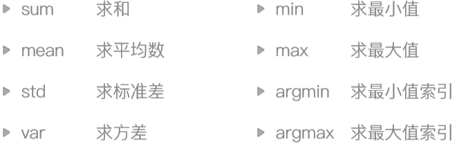
数组排序
# 生成示例数组
a = np.array(([1, 4, 3], [6, 2, 9], [4, 7, 2]))
a
array([[1, 4, 3],
       [6, 2, 9],
       [4, 7, 2]])

#  返回每列最大值
np.max(a, axis=0)
array([6, 7, 9])

# 返回每行最小值
np.min(a,axis=1)
array([1, 2, 2])

# 返回每列最大值索引
np.argmax(a,axis=0)
array([1, 2, 1])

# 返回每行最小值索引
np.argmin(a,axis=1)
array([0, 1, 2])
numpy-统计方法和随机数生成
# 统计中位数
np.median(a, axis=0)

# 统计各行的算术平均值
np.mean(a, axis=1)

# 统计各列的加权平均值
np.average(a, axis=0)

# 统计各行的方差
np.var(a, axis=1)

# 统计数组各列的标准偏差
np.std(a, axis=0)
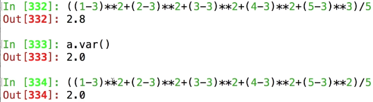
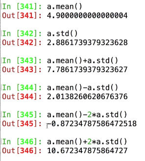
数学时间
1 2 3 4 5
平均数: 3
方差 :每个数-3的值的平方,加在一起,再除以数字的个数
方差用来计算数组内数值的范围
平均数加减两倍方差的结果活落在90%的范围上
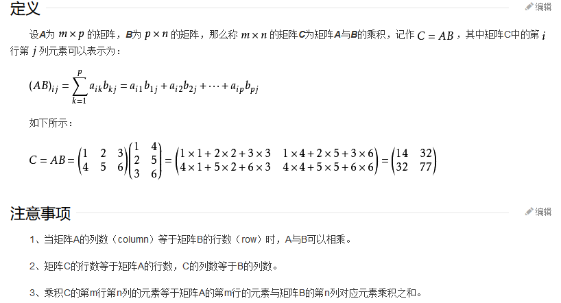
矩阵乘法
矩阵乘法运算(注意与a*b的区别)
A = np.array([[1,2],[3,4]])
B = np.array([[5,6],[7,8]])

np.dot(A,B)
array([[19, 22],
       [43, 50]])
数学函数
# 求三角函数
a = np.array([10,20,30,40,50])

np.sin(a)
array([-0.54402111,  0.91294525, -0.98803162,  0.74511316, -0.26237485])

#   以自然对数为底数的指数函数
np.exp(a)
array([2.20264658e+04, 4.85165195e+08, 1.06864746e+13, 2.35385267e+17,
       5.18470553e+21])

# 方根的运算-开平方
np.sqrt(a)
array([3.16227766, 4.47213595, 5.47722558, 6.32455532, 7.07106781])

# 方根的运算-求立方
np.power(a,3)
array([  1000,   8000,  27000,  64000, 125000])
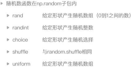
随机数
# 创建二维随机数组
np.random.rand(2, 3)
array([[0.46181641, 0.06400509, 0.93763711],
       [0.67133387, 0.0801051 , 0.81633397]])

# 创建二维随机整数数组
np.random.randint(5, size=(2, 3))
array([[4, 2, 2],
       [4, 0, 0]])
In [61]: np.random.randint(0,10,10)
Out[61]: array([6, 4, 8, 4, 0, 4, 9, 1, 5, 7])
# 生成多维随机数组
In [62]: np.random.randint(0,10,(3,5))   或者如上一个例子所示 使用size参数
Out[62]:
array([[4, 5, 7, 7, 8],
       [4, 1, 5, 1, 4],
       [2, 3, 9, 6, 8]])

# 0-1之间的随机数
In [63]: np.random.rand(10)
Out[63]:
array([0.97926997, 0.17454168, 0.52831388, 0.28070782, 0.2715298 ,
       0.2749287 , 0.44007621, 0.56472258, 0.53291951, 0.30727733])

# 指定数组中的随机数
In [64]: np.random.choice([1,2,3,4,5,6],10)
Out[64]: array([1, 2, 5, 5, 2, 1, 5, 1, 3, 1])

In [65]: np.random.choice([1,2,3,4,5,6],(2,3))
Out[65]:
array([[5, 2, 3],
       [3, 4, 4]])

# uniform 平均分布,出现每一个小数的概率都一样
In [67]: np.random.uniform(2.0,4.0,10)
Out[67]:
array([3.30135597, 2.5034658 , 3.80415042, 3.58323964, 2.82819204,
       3.45701693, 2.51628589, 3.94588971, 2.46530701, 3.269412  ])

In [68]: np.random.uniform(2,4,10)
Out[68]:
array([3.99532675, 2.27704994, 2.44378248, 2.33492658, 3.79537452,
       2.6754694 , 3.04022564, 2.12863367, 3.27047096, 3.70261513])

In [69]: # random中所有的方法都被numpy重写过
fromfunction-依据自定义函数创建数组
>>> def f(x,y):
...         return 10*x+y
...
>>> b = fromfunction(f,(5,4),dtype=int)
>>> b
array([[ 0,  1,  2,  3],
        [10, 11, 12, 13],
        [20, 21, 22, 23],
        [30, 31, 32, 33],
        [40, 41, 42, 43]])

#
np.fromfunction(lambda i,j:i+j,(3,3))
array([[0., 1., 2.],
       [1., 2., 3.],
       [2., 3., 4.]])
# 生成的规则就是数组中每一个元素所在位置的索引值作为x和y的值
还有很多高级功能没有说,numpy相对于pandas来说是比较基础的包
接下来请领教pandas
第三章-数据分析核心包---pandas
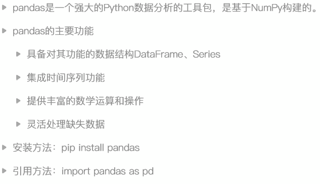
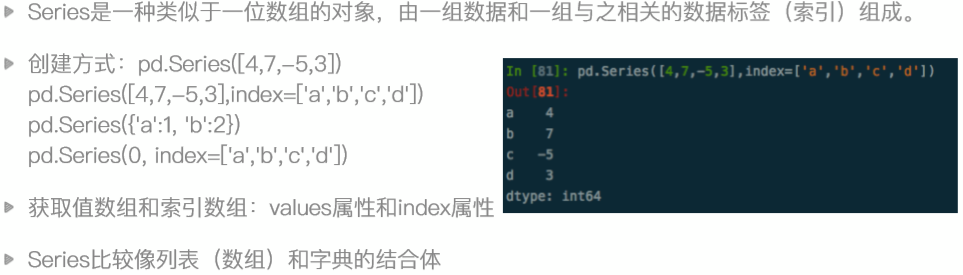
series-一维数据对象
In [72]: import pandas as pd

In [73]: pd.Series([2,3,4,5])
Out[73]:
0    2
1    3
2    4
3    5
dtype: int64

In [74]: pd.Series([2,3,4,5],index=['a','b','c','d'])
Out[74]:
a    2
b    3
c    4
d    5
dtype: int64

In [75]: # 所以说serries更像是列表和字典的结合体

In [76]: pd.Series(np.arange(5))
Out[76]:
0    0
1    1
2    2
3    3
4    4
dtype: int32

In [77]: # 在制定了索引之后,用原来的下标还是能访问
In [82]:  sr = pd.Series([2,3,4,5],index=['a','b','c','d'])

In [83]: sr
Out[83]:
a    2
b    3
c    4
d    5
dtype: int64

In [84]: sr[2]
Out[84]: 4
# 所以他有两种索引方式,一种是下标,一种是标签,像字典的key
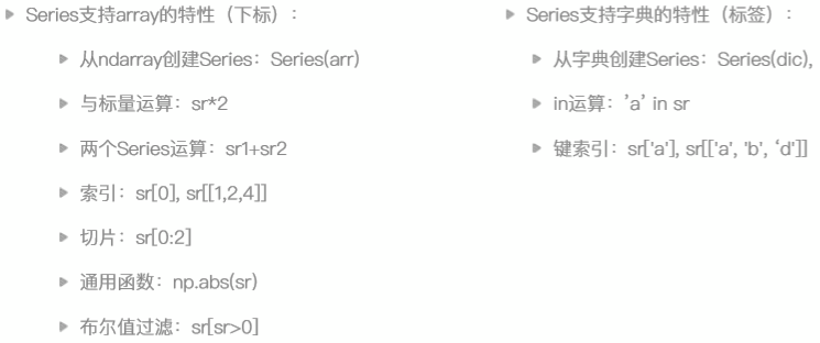
Series-使用特性
# 字典创建Series
In [85]: sr = pd.Series({'a':1,'b':2})
In [86]: sr
Out[86]:
a    1
b    2
# 键索引
dtype: int64
In [88]: sr['a']
Out[88]: 1
# in的用法
In [89]: 'a' in sr
Out[89]: True
# 通过字典创建,也能使用下标索引
In [87]: sr[1]
Out[87]: 2
# 和字典有一点不一样,写for循环的时候,for字典循环的是key,而Series遍历的是值
In [90]: for i in sr:
    ...:     print(i)
    ...:
1
2

# 获取索引
In [91]: sr.index
Out[91]: Index(['a', 'b'], dtype='object')
In [93]: sr.index[0]
Out[93]: 'a'
# 获取值
In [94]: sr.values
Out[94]: array([1, 2], dtype=int64)

In [95]: sr.values[0]
Out[95]: 1
# 花式索引
In [101]: sr = pd.Series(a,index=['a','b','c','d','e'])

In [102]: sr
Out[102]:
a    3
b    4
c    5
d    6
e    7
dtype: int32

In [103]: sr[['a','e','c']]
Out[103]:
a    3
e    7
c    5
dtype: int32
# 标签索引来切片,它是前包后也包的
In [106]: sr['b':'d']
Out[106]:
b    4
c    5
d    6
dtype: int32
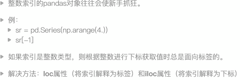
Series-整数索引问题
In [107]: sr = pd.Series(np.arange(10))

In [108]: sr
Out[108]:
0    0
1    1
2    2
3    3
4    4
5    5
6    6
7    7
8    8
9    9
dtype: int32

In [111]: sr2 = sr[5:].copy()
In [112]: sr2
Out[112]:
5    5
6    6
7    7
8    8
9    9
dtype: int32
# 问题开始了,sr2的下标索引并不是从0开始的
In [113]: sr2[5]
Out[113]: 5
# 因为这个时候是有歧义的,所以,如果索引是整数类型,则根据整数进行下标取值的时候,总是面相标签的
解决办法:loc和iloc
In [114]: sr2.loc[5]
Out[114]: 5

In [115]: sr2.iloc[-1]
Out[115]: 9
# 因为长度只有5,所以使用sr.iloc[5]会报错
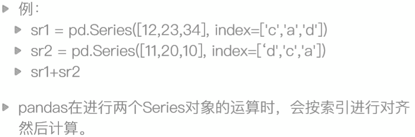
Series-数据对齐
按照标签索引进行计算
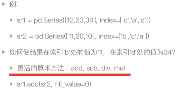
In [117]: sr1 = pd.Series([12,23,34],index=['c','a','d'])
In [118]: sr2 = pd.Series([11,20,10],index=['d','c','a'])

In [119]: sr1+sr2
Out[119]:
a    33
c    32
d    45
dtype: int64
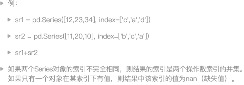
pandas中长度不一样也可以计算,并引入NaN数据作为数据缺失值
In [120]: sr1 = pd.Series([12,23,34],index=['c','a','d'])

In [121]: sr2 = pd.Series([11,20,10,16],index=['d','c','a','b'])

In [122]: sr1+sr2
Out[122]:
a    33.0
b     NaN
c    32.0
d    45.0
dtype: float64
In [123]: sr1 = pd.Series([12,23,34],index=['c','a','d'])

In [124]: sr2 = pd.Series([11,20,10],index=['c','a','b'])

In [125]: sr1+sr2
Out[125]:
a    43.0
b     NaN
c    23.0
d     NaN
dtype: float64
但是有的时候,我不需要他出现NaN
In [126]: sr1.add(sr2,fill_value=0)
Out[126]:
a    43.0
b    10.0
c    23.0
d    34.0
dtype: float64
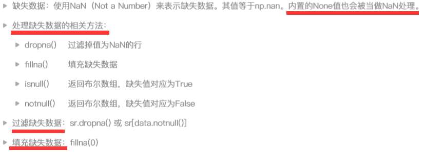
Series-缺失数据和处理确实数据
处理缺失数据有两种思路-删除和填充
判断有没有缺失数据-isnull和notnull
In [127]: sr.isnull()
Out[127]:
0    False
1    False
2    False
dtype: bool
删掉缺失数据的方法
# 恶意直接利用索引取值的方法
In [132]: sr[sr.notnull()]
Out[132]:
a    43.0
c    23.0
dtype: float64
# 使用dropna 删除
In [134]: sr.dropna()
Out[134]:
a    43.0
c    23.0
dtype: float64
填充的方法
# 使用fillna填充
In [133]: sr.fillna(0)
Out[133]:
a    43.0
b     0.0
c    23.0
d     0.0
dtype: float64
有的时候,不喜欢看见0 ,我们可以填充一个平均值
In [135]: sr.fillna(sr.mean())
Out[135]:
a    43.0
b    33.0
c    23.0
d    33.0
dtype: float64
pandas在计算平均值的时候,会跳过nan。如果不想跳过去,可以加一些参数
Series小结
Series的特性-数组+字典的结合体-
整数索引的问题-loc和iloc
数据对齐-面向标签和缺失值
缺失值的处理-删除和填充
pandas的mean求平均值的特点的使用
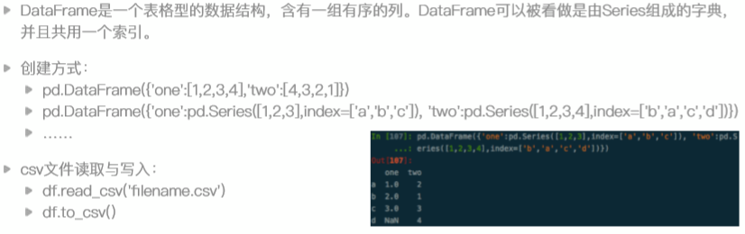
DataFrame-二维数据对象
# 第一种创建范式
In [137]: df=pd.DataFrame({'one':[1,2,3,],'two':[4,5,6]})

In [138]: df
Out[138]:
   one  two
0    1    4
1    2    5
2    3    6
# 第二种创建方式
In [140]: pd.DataFrame({'one':pd.Series([1,2,3],index=['a','b','c']),'two':pd.Series([4,5,6,7],index=['a','b','c','d'])})
Out[140]:
   one  two
a  1.0    4
b  2.0    5
c  3.0    6
d  NaN    7
# 还有很多种创建的方式...
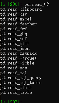
文件读写操作
vim test.csv
读取csv文件
In [145]: pd.read_csv('test.csv')
Out[145]:
   a  b  c
0  1  2  3
1  4  5  6
2  7  8  9
保存文件为csv
In [147]: df
Out[147]:
   a  b  c
0  1  2  3
1  4  5  6
2  7  8  9

In [148]: df.to_csv('test2.csv')
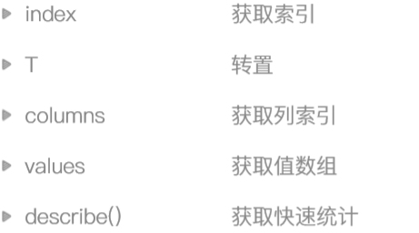
DataFrame-常用属性
index用来获取行索引,values获取的值是二维数组, 这是和Series一样的地方
In [156]: df = _140

In [157]: df
Out[157]:
   one  two
a  1.0    4
b  2.0    5
c  3.0    6
d  NaN    7

In [158]: df.index
Out[158]: Index(['a', 'b', 'c', 'd'], dtype='object')

In [159]: df.values
Out[159]:
array([[ 1.,  4.],
       [ 2.,  5.],
       [ 3.,  6.],
       [nan,  7.]])
转置T-把行变成列,列变成行,且一列都成了一个属性(所有的转置默认都会)
可以指定属性dtype
In [160]: df.T
Out[160]:
       a    b    c    d
one  1.0  2.0  3.0  NaN
two  4.0  5.0  6.0  7.0
获取列索引columns
In [163]: df.columns
Out[163]: Index(['one', 'two'], dtype='object')
快速统计
In [165]: df.describe()
Out[165]:
       one       two
count  3.0  4.000000  个数
mean   2.0  5.500000  平均数
std    1.0  1.290994  标准差
min    1.0  4.000000  最小值
25%    1.5  4.750000  25%位置的数
50%    2.0  5.500000  中位数
75%    2.5  6.250000  75%位置的数
max    3.0  7.000000  最大数
DataFrame-索引和切片
# 先选列。再选行
In [168]: df
Out[168]:
   one  two
a  1.0    4
b  2.0    5
c  3.0    6
d  NaN    7

In [169]: df['one']['a']
Out[169]: 1.0

In [170]: df['one'][1]
Out[170]: 2.0

In [171]: df['one'][0]
Out[171]: 1.0
建议使用loc或者iloc指定,并不建议使用双中括号
In [172]: df.loc['a','one']
Out[172]: 1.0

In [173]: df.loc['a',:]
Out[173]:
one    1.0
two    4.0
Name: a, dtype: float64
灵活搭配使用
In [174]: df.loc[['a','c'],:]
Out[174]:
   one  two
a  1.0    4
c  3.0    6
DataFrame-数据对齐与缺失数据
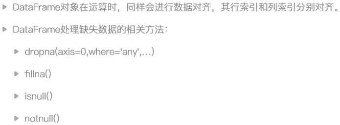
DataFrame在使用dropna时,如果一行有一个缺失值,会将整行都删除
指定how=‘all’,删除全部是nan的行
In [177]: df.loc[['c','d'],'two'] = np.nan

In [178]: df
Out[178]:
   one  two
a  1.0  4.0
b  2.0  5.0
c  3.0  NaN
d  NaN  NaN

In [179]: df.dropna(how='all')
Out[179]:
   one  two
a  1.0  4.0
b  2.0  5.0
c  3.0  NaN
# how 默认的值是any,也就是只要有nan就都会删除
如何把有一列中有缺失值的那一列都删除?
axis参数意思是-轴,默认是0,是0的时候,指定的是行,1指定的是列
In [184]: df
Out[184]:
   one  two
a  1.0  4.0
b  2.0  5.0
c  3.0  NaN
d  5.0  NaN

In [185]: df.dropna(axis=1)
Out[185]:
   one
a  1.0
b  2.0
c  3.0
d  5.0
pandas-其他常用方法
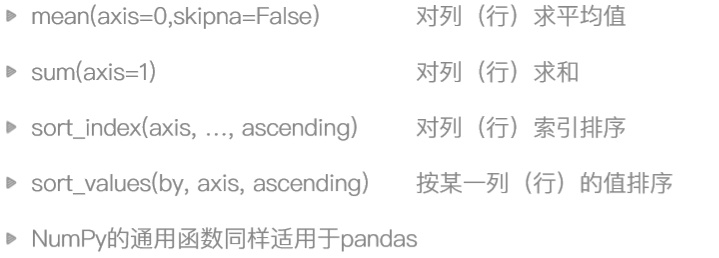
排序中的ascending=False是倒序,by是指定排序的行(列)
当排序的列(行)有nan的时候,都默认放在了最后,不参与排序
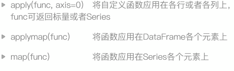
numpy的所有通用函数都适于用pandas
pandas-时间对象处理
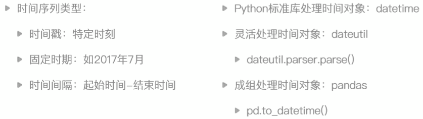
datetime中将时间字符串转化成时间对象
In [186]: import datetime

In [187]: datetime.datetime.strptime('2010-01-01','%Y-%m-%d')
Out[187]: datetime.datetime(2010, 1, 1, 0, 0)
记忆strptime   p--parse 解析
记忆strftime   f--format 格式化
但是不是所有人写时间的格式都像这样的,有一个库可以帮我们做这件事
import  dateutil

In [191]: dateutil.parser.parse('02/03/2010')
Out[191]: datetime.datetime(2010, 2, 3, 0, 0)

In [192]: dateutil.parser.parse('02-03-2010')
Out[192]: datetime.datetime(2010, 2, 3, 0, 0)

In [193]: dateutil.parser.parse('2010-JAN-10')
Out[193]: datetime.datetime(2010, 1, 10, 0, 0)
pandas中的to_datetime就是引用了这个模块,进行批量转换
In [194]: pd.to_datetime(['02-03-2010','2010-JAN-10'])
Out[194]: DatetimeIndex(['2010-02-03', '2010-01-10'], dtype='datetime64[ns]', freq=None)
注意:得到对象第DatetimeIndex
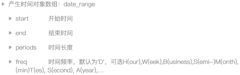
时间对象生成-date_range
In [195]: pd.date_range('2010-01-01','2010-05-01')
Out[195]:
DatetimeIndex(['2010-01-01', '2010-01-02', '2010-01-03', '2010-01-04',
               '2010-01-05', '2010-01-06', '2010-01-07', '2010-01-08',
               '2010-01-09', '2010-01-10',
               ...
               '2010-04-22', '2010-04-23', '2010-04-24', '2010-04-25',
               '2010-04-26', '2010-04-27', '2010-04-28', '2010-04-29',
               '2010-04-30', '2010-05-01'],
              dtype='datetime64[ns]', length=121, freq='D')
使用periods指定长度
pd.date_range? 查看帮助中的参数帮助信息
start : str or datetime-like, optional
    Left bound for generating dates.
end : str or datetime-like, optional
    Right bound for generating dates.
periods : integer, optional   长度
    Number of periods to generate.
freq : str or DateOffset, default 'D'  频率 H-小时 W-周 W-MON W-WEN
    Frequency strings can have multiples, e.g. '5H'. See  //B-工作日
    :ref:`here <timeseries.offset_aliases>` for a list of //1H20min
    frequency aliases.
date_range的参数freq可以各种花式定义时间间隔
tz : str or tzinfo, optional
    Time zone name for returning localized DatetimeIndex, for example
    'Asia/Hong_Kong'. By default, the resulting DatetimeIndex is
    timezone-naive.
normalize : bool, default False
    Normalize start/end dates to midnight before generating date range.
name : str, default None
    Name of the resulting DatetimeIndex.
closed : {None, 'left', 'right'}, optional
    Make the interval closed with respect to the given frequency to
    the 'left', 'right', or both sides (None, the default).
得到的是Timestamp对象,可以将其用to_pydatetime转换成时间对象
还可以转成字符串
date_range的参数freq可以各种花式定义时间间隔
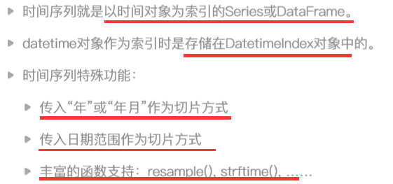
时间序列
生成的时间对象可以用来构建时间序列的
In [198]: sr = pd.Series(np.arange(5),index=pd.date_range('2010-01-01',periods=5))

In [199]: sr
Out[199]:
2010-01-01    0
2010-01-02    1
2010-01-03    2
2010-01-04    3
2010-01-05    4
Freq: D, dtype: int32
那么有什么作用呢?直观的好处就是以时间为索引获取指定范围的数据
In [200]: sr = pd.Series(np.arange(100),index=pd.date_range('2010-01-01',periods=100))

In [201]: sr['2010-03']
Out[201]:
2010-03-01    59
2010-03-02    60
2010-03-03    61
2010-03-04    62
2010-03-05    63
2010-03-06    64
2010-03-07    65
2010-03-08    66
2010-03-09    67
2010-03-10    68
2010-03-11    69
2010-03-12    70
2010-03-13    71
2010-03-14    72
2010-03-15    73
2010-03-16    74
2010-03-17    75
2010-03-18    76
2010-03-19    77
2010-03-20    78
2010-03-21    79
2010-03-22    80
2010-03-23    81
2010-03-24    82
2010-03-25    83
2010-03-26    84
2010-03-27    85
2010-03-28    86
2010-03-29    87
2010-03-30    88
2010-03-31    89
Freq: D, dtype: int32
还比如 sr['2017':'2018']
特别方便
resample函数--重新取样
# 以周为单位取和
In [203]: sr.resample('W').sum()
Out[203]:
2010-01-03      3
2010-01-10     42
2010-01-17     91
2010-01-24    140
2010-01-31    189
2010-02-07    238
2010-02-14    287
2010-02-21    336
2010-02-28    385
2010-03-07    434
2010-03-14    483
2010-03-21    532
2010-03-28    581
2010-04-04    630
2010-04-11    579
Freq: W-SUN, dtype: int32
truncate是类似切片的函数,意义不大,因为都可以通过切片操作来取值
pandas-文件处理
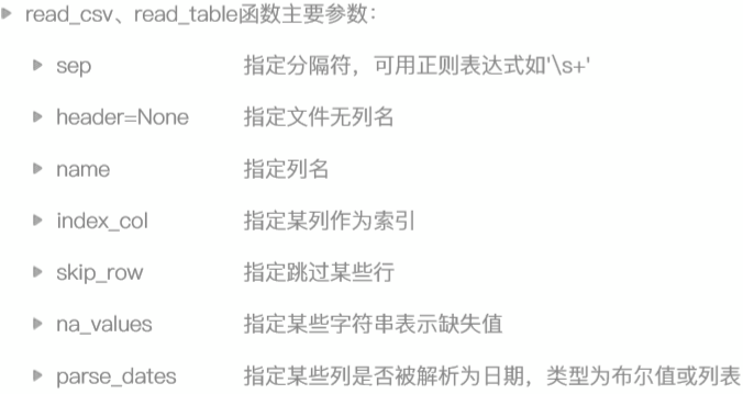
读取文件
例子:
header= none
names的使用
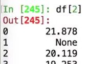
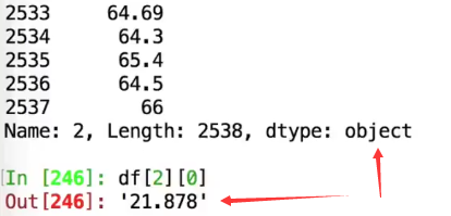
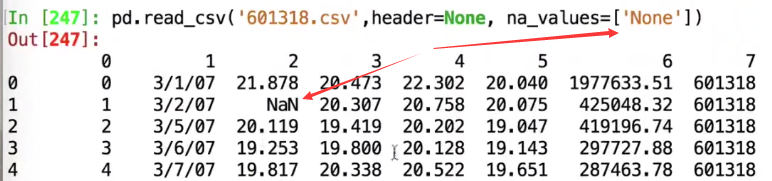
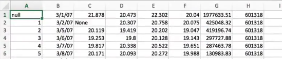
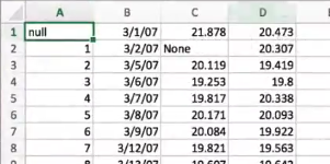
在一个数据表中,如果某一列中有None,这整个列的类型都会变成object,变成了字符串
本来应该是float的
但是因为有none,变成了字符串
nan可以解释成浮点数,但是none无法解释,
解决:用na_values
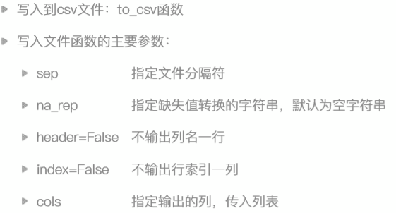
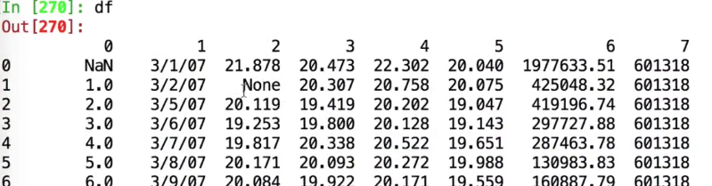
写入文件
写入文件示例:
Python中读取excel的时候需要安装模块xlrd
......还有很多内容
要多多练习,才能掌握,变成自己的
第四章-数据可视化工具包---matplotlib
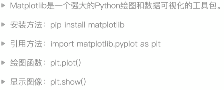
如果在命令行或者pycharm中运行,会弹出对话框,可以进行拖动、放大等操作...
plot函数
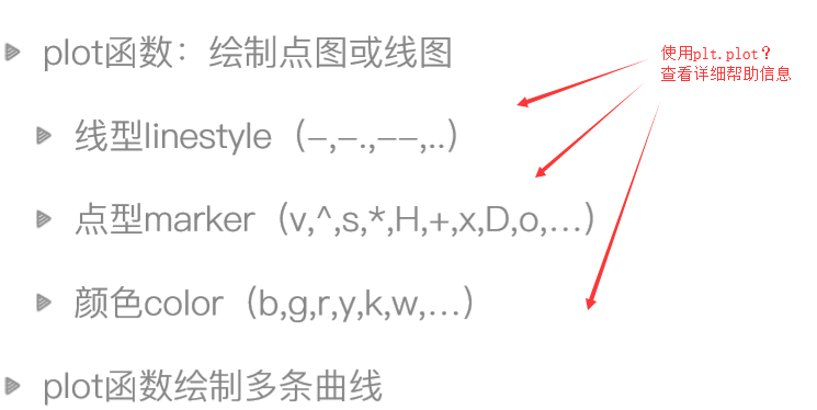
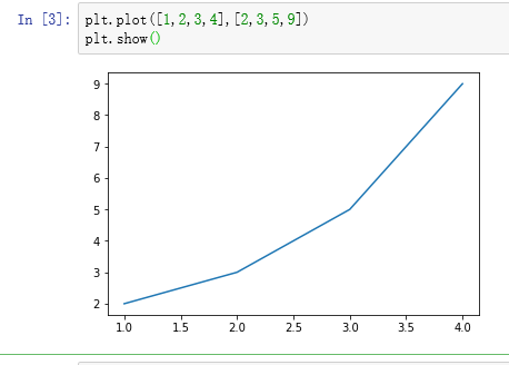
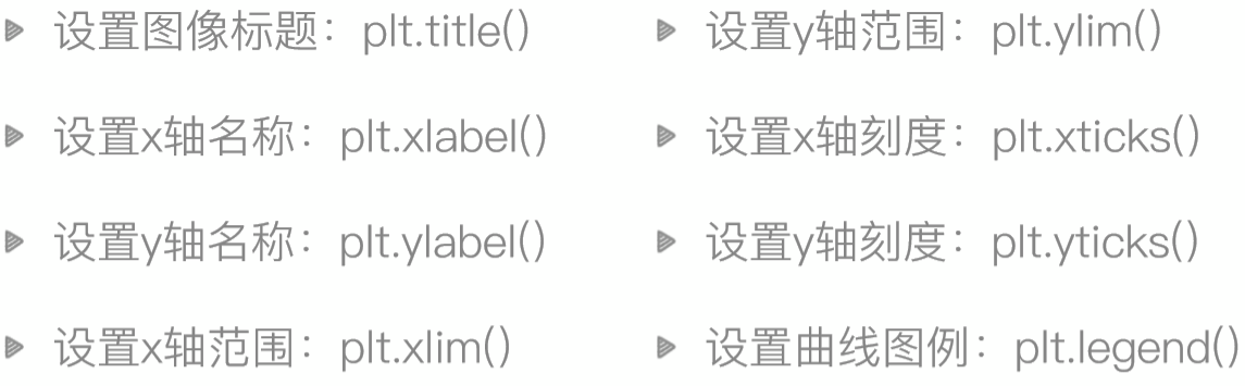
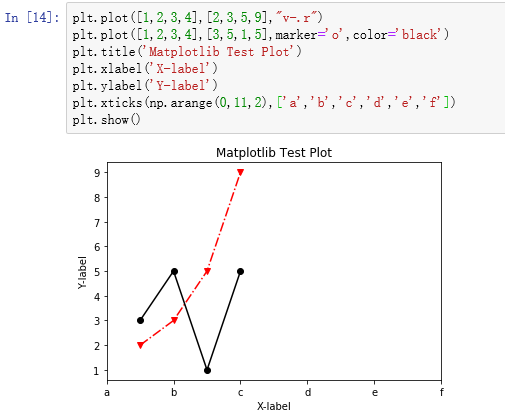
plot用来绘制点图或者线图,两个参数(即x和y)
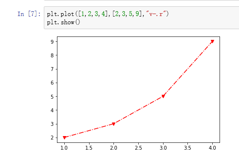
还有第三个参数,一个字符串,来决定线的样式(示例:v是小三角,用短线和点连接,显示红色)
也可以使用参数传递(color=‘red’,marker=‘^’,linestyle='-.')
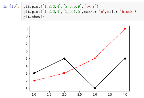
我想画多条线?该如何操作
show函数,调用之后,之前的plot都出现在一张图上了
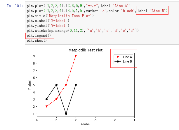
Matplotlib-图像标注
plt.legend的用法之一
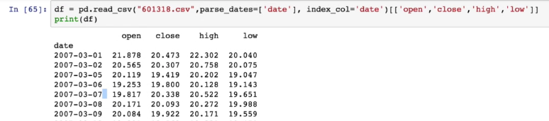
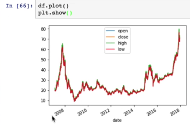
pandas和Matplotlib
直接使用
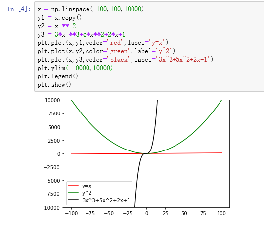
作业:绘制数学函数图像
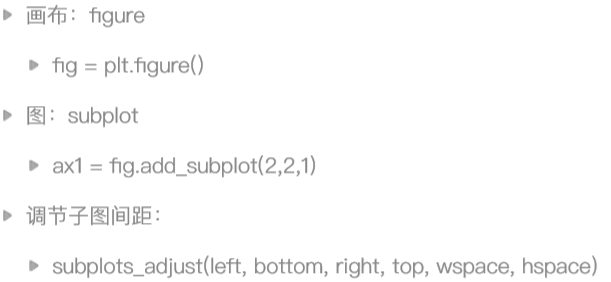
画布与子图
fig.add_subplot(2,2,1) 其中 2,2的意思就是把画布分成2x24份,最后的1是第一个位置
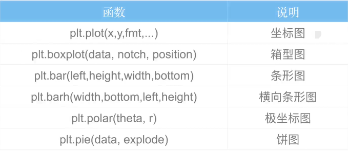
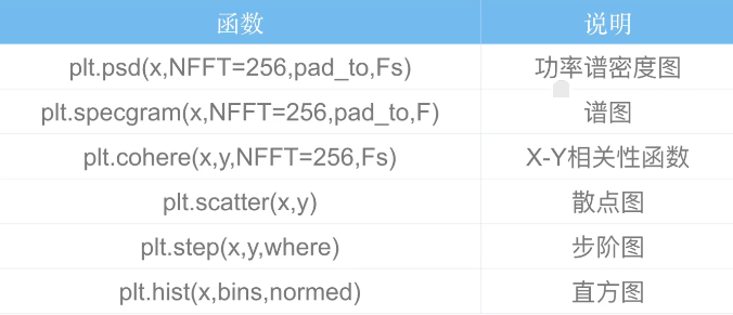
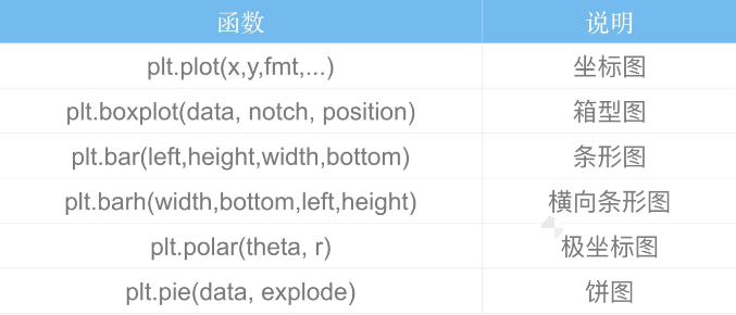
Matplotlib支持的图类型
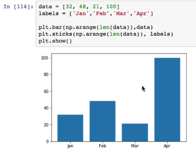
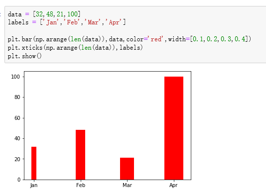
条形图
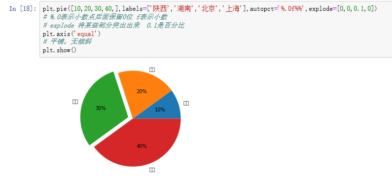
饼图
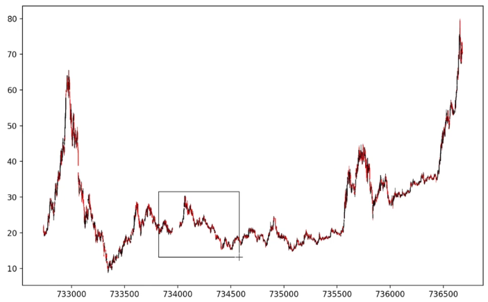
折线图-matplot.finance
matplotlib.finance.子包中有许多绘制金融相关图的函数接口
绘制K线图:matplotlib.finance.candlestick_ochl函数
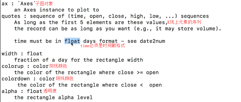
参数的帮助信息
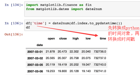
导入模块并给数据添加了一个time字段
第五章-金融数据分析基础实战
tushare包介绍
Tushare是一个免费、开源的财经数据接口包。
练习1-股票数据分析
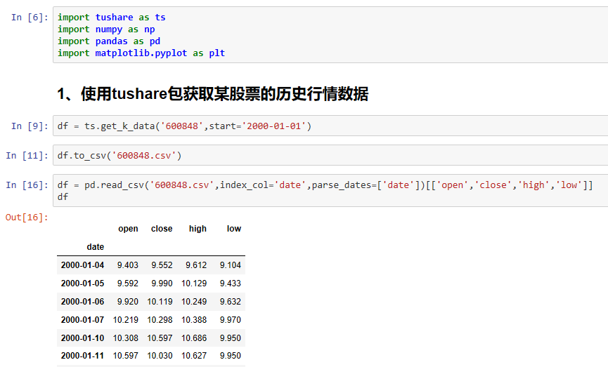
1、使用tushare包获取某股票的历史行情数据
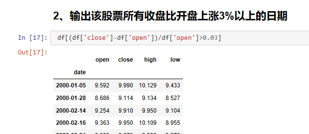
2、输出该股票所有收盘比开盘上涨3%以上的日期
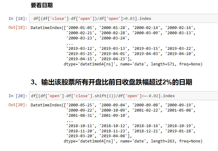
3、输出该股票所有开盘比前日收盘跌幅超过2%的日期(用shift错位)
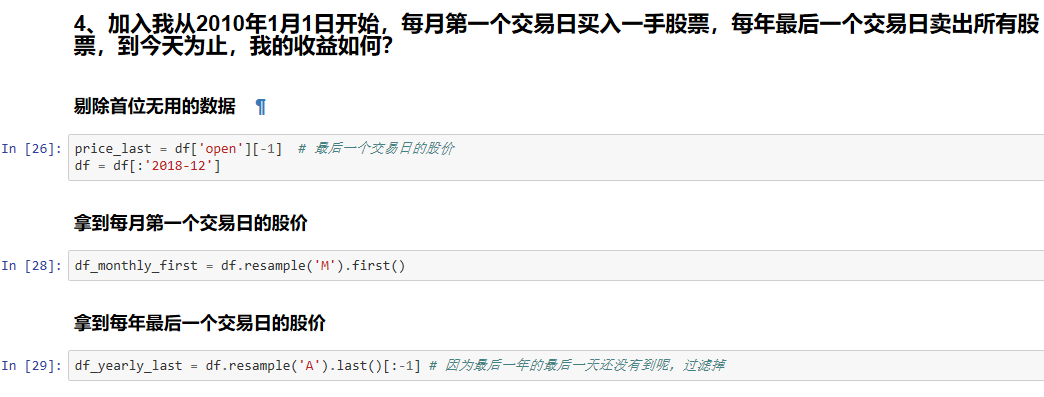
4、加入我从2010年1月1日开始,每月第一个交易日买入一手股票,每年最后一个交易日卖出所有股票,
到今天为止,我的收益如何?
tushare接口的使用和shift函数,resample的使用
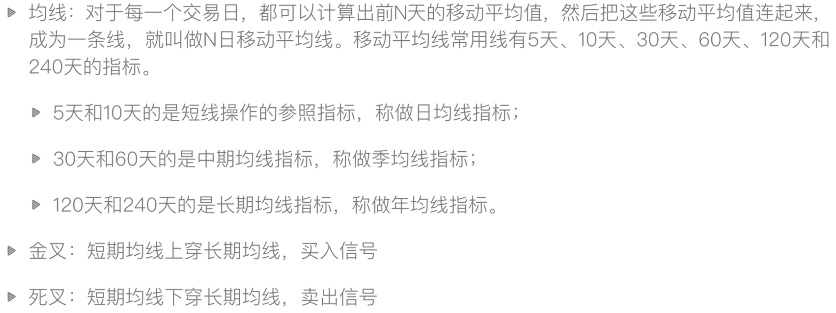
练习2-查找历史金叉死叉的日期
编写代码
第一个量化策略
基于聚宽编码和回测
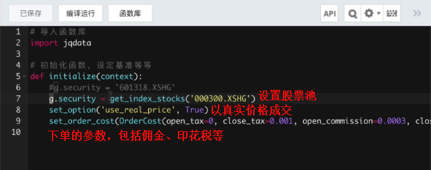
initialize函数
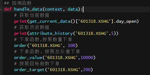
handle_data函数,每个单位时间执行一次回测
策略实现
# 导入函数库
from jqdata import *

# 初始化函数,设定基准等等
def initialize(context):
    # 1、设置股票池为沪深300的所有成分股
    g.security = get_index_stocks('000300.XSHG')
   # 基准收益
    set_benchmark('000300.XSHG') # 持有后不动
    set_option('use_real_price',True)
    set_order_cost(OrderCost(open_tax=0, close_tax=0.001, open_commission=0.0003, close_commission=0.0003, close_today_commission=0, min_commission=5), type='stock')
## 回测函数
def handle_data(context, data):
    # 每只股票买多少的问题,账户金额/股票个数的长度=每个股票分多少钱

    # 一般情况下先卖后买
    tobuy = []
    for stock in g.security:
        # 获取股票当前的开盘价
        p = get_current_data()[stock].day_open
        # 查看是否持有这只股票
        amount = context.portfolio.positions[stock].total_amount
        # 股票的持仓成本
        cost = context.portfolio.positions[stock].avg_cost
        # 3、如果当前股价比买入时上涨了25%,则清仓止盈
        if amount > 0 and p >= cost * 1.25:
            order_target(stock,0)  # 止盈
        # 4、如果当前股价比买入时下跌了10%,则卖出止损
        if amount > 0 and p <= cost *0.9:
            order_target(stock,0)  # 止损
        # 2、如果当前股价小于10元且当前不持仓,则买入
        if p <= 10.0 and amount == 0:
            tobuy.append(stock)
            order(stock,1000)
        if tobuy:
            cost_per_stock = context.portfolio.available_cash / len(tobuy)
            for per in tobuy:
                order_value(per,cost_per_stock)
双均线策略-最简单只股票
# 导入函数库
from jqdata import *

# 初始化函数,设定基准等等
def initialize(context):
    set_benchmark('000300.XSHG') # 持有后不动
    set_option('use_real_price',True)
    set_order_cost(OrderCost(open_tax=0, close_tax=0.001, open_commission=0.0003, close_commission=0.0003, close_today_commission=0, min_commission=5), type='stock')

    # 选股
    g.security = ['601318.XSHG']
    g.p1 = 5
    g.p2 = 10


def handle_data(context, data):
    for stock in g.security:
        # 金叉:如果5日均线大于10日均线,且没有持仓
        # 死叉:如果5日均线小于10日均线,并且持仓
        # 获取历史数据
        df = attribute_history(stock,g.p2)
        m10 = df['close'].mean()
        m5 = df['close'][-5:].mean()

        if m10 > m5 and stock in context.portfolio.positions:
            # 死叉卖出
            order_target(stock, 0)
        if m10 < m5 and stock not in context.portfolio.positions:
            order(stock,context.portfolio.available_cash * 0.8)
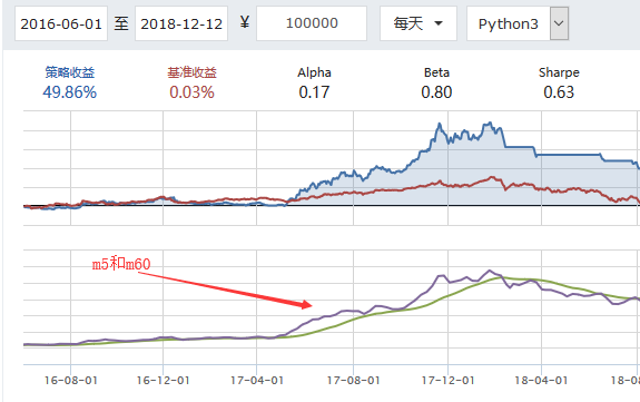
在回测图上添加其他的图
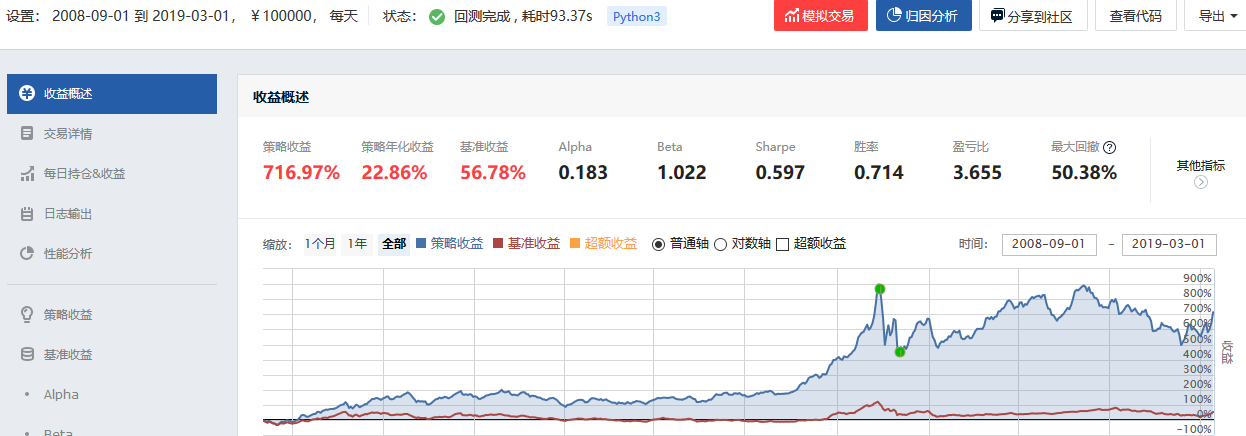
因子选股策略
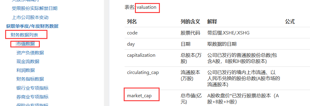
查询财务数据
get_fundanmentals
策略编写
# 导入函数库
from jqdata import *

# 初始化函数,设定基准等等
def initialize(context):
    set_benchmark('000300.XSHG') # 持有后不动
    set_option('use_real_price',True)
    set_order_cost(OrderCost(open_tax=0, close_tax=0.001, open_commission=0.0003,
    close_commission=0.0003, close_today_commission=0, min_commission=5), type='stock')

    # 选股范围
    g.security = get_index_stocks('000300.XSHG')

    # 获取数据,在官网数据选项卡中找到valuation表
    g.q = query(valuation).filter(valuation.code.in_(g.security))

    # 要定期跟新调仓
        # 1、定义天数变量,在handle_data中计数,每天+1,当days%30==0的时候,执行调仓
            # 这是没30个交易日调一次
        # 2、使用run_monthly(handle,1),定义handle用来跟新的函数,1表示第一个交易日
            # 这是每月调一次
    run_monthly(handle,1)

    # 定义自己的仓位最多有20只股票
    g.N = 20
def handle(context):
    # 注意,有的函数方法会报错,因为平台支持的第三方平台的版本所导致
    df = get_fundamentals(g.q)[['code','market_cap']]
    df = df.sort_values('market_cap').iloc[:g.N,:]
    # 新选出的股票池
    to_hold = df['code'].values

    # 手上可能有一些股票,有的留着,没有的卖掉,添加新的
    for stock in context.portfolio.positions:
        # 手上的股票没在to_hold中,买掉
        if stock not in to_hold:
            order_target(stock,0)

    to_buy = [stock for stock in to_hold if stock not in context.portfolio.positions]

    if to_buy:
        cash_per_stock = context.portfolio.available_cash / len(to_buy)
        for per in to_buy:
            order_value(per,cash_per_stock)
注意停牌的股票的过滤
取前30个,把停牌的(paused)过滤掉,在取前20个
多因子选股策略
市值小
净资产收益率要高
如何同时综合多个因子
...
补充知识-标准化
标准化,归一化,数据预处理的方法
编码实现
# 导入函数库
from jqdata import *

# 初始化函数,设定基准等等
def initialize(context):
    set_benchmark('000300.XSHG') # 持有后不动
    set_option('use_real_price',True)
    set_order_cost(OrderCost(open_tax=0, close_tax=0.001, open_commission=0.0003,
    close_commission=0.0003, close_today_commission=0, min_commission=5), type='stock')

    # 选股范围
    g.security = get_index_stocks('000002.XSHG')

    # 获取数据,在官网数据选项卡中找到valuation表,市值数据在这个表中
    # 找到roe在,indicator表中
    g.q = query(valuation,indicator).filter(valuation.code.in_(g.security))


    # 要定期跟新调仓
        # 1、定义天数变量,在handle_data中计数,每天+1,当days%30==0的时候,执行调仓
            # 这是没30个交易日调一次
        # 2、使用run_monthly(handle,1),定义handle用来跟新的函数,1表示第一个交易日
            # 这是每月调一次
        # 定义自己的仓位最多有20只股票
    g.N = 20

    run_monthly(handle,1)


def handle(context):
    # 注意,有的函数方法会报错,因为平台支持的第三方平台的版本所导致
    df = get_fundamentals(g.q)[['code','market_cap','roe']]
    # 进行归一化
    df['market_cap'] = (df['market_cap']) - df['market_cap'].min()) / (df['market_cap'].max() - df['market_cap'].min())
    df['roe'] = (df['roe']) - df['roe'].min()) / (df['roe'].max() - df['roe'].min())
    # 增加一列作为评分,收益率越大越好,市值越小越好。最后的结果越大越好
    df['score'] = df['roe'] - df['market_cap']
    # 选最后20只
    df = df.sort_values('score').iloc[-g.N:,:]

    # 新选出的股票池
    to_hold = df['code'].values

    # 手上可能有一些股票,有的留着,没有的卖掉,添加新的
    for stock in context.portfolio.positions:
        # 手上的股票没在to_hold中,买掉
        if stock not in to_hold:
            order_target(stock,0)

    to_buy = [stock for stock in to_hold if stock not in context.portfolio.positions]

    if to_buy:
        cash_per_stock = context.portfolio.available_cash / len(to_buy)
        for per in to_buy:
            order_value(per,cash_per_stock)
还可以增加权重、增加更多的因子
均值回归理论
均值回归策略是一个选股策略
编码实现
# 导入函数库
from jqdata import *

# 初始化函数,设定基准等等
def initialize(context):
    set_benchmark('000300.XSHG') # 持有后不动
    set_option('use_real_price',True)
    set_order_cost(OrderCost(open_tax=0, close_tax=0.001, open_commission=0.0003,
    close_commission=0.0003, close_today_commission=0, min_commission=5), type='stock')

    # 选股范围
    g.security = get_index_stocks('000002.XSHG')

    # 均线
    g.ma_days = 30

    # 股票数量
    g.stock_num = 10

    run_monthly(handle,1)

def handle(context):
    sr = pandas.Series(index=g.security)
    for stock in sr.index:
        ma = attribute_history(stock, g.ma_days)['close'].mean()
        p = get_current_data()[stock].day_open
        # 计算偏离程度
        ratio = (ma-p) / ma
        sr[stock] = ratio

    # 不用sort,有一个更快的函数nlargest
    # 新选出的股票池
    to_hold = sr.nlargest(g.stock_num).index.values

    # 手上可能有一些股票,有的留着,没有的卖掉,添加新的
    for stock in context.portfolio.positions:
        # 手上的股票没在to_hold中,买掉
        if stock not in to_hold:
            order_target(stock,0)

    to_buy = [stock for stock in to_hold if stock not in context.portfolio.positions]

    if to_buy:
        cash_per_stock = context.portfolio.available_cash / len(to_buy)
        for per in to_buy:
            order_value(per,cash_per_stock)
布林带策略
上下N取小了不好,去大了等于没取,因为很难触碰,上下可以取不同的N
编码实现
# 导入函数库
from jqdata import *

# 初始化函数,设定基准等等
def initialize(context):
    set_benchmark('000300.XSHG') # 持有后不动
    set_option('use_real_price',True)
    set_order_cost(OrderCost(open_tax=0, close_tax=0.001, open_commission=0.0003,
    close_commission=0.0003, close_today_commission=0, min_commission=5), type='stock')

    # 选股范围
    g.security = ('600036.XSHG')

    g.M = 20  # 试验过20比较好
    g.k = 2  # 听说1.7比较好
# 初始化策略
def handle_data(context, data):
    sr = attribute_history(g.security,g.M)['close']
    ma = sr.mean()
    up = ma + g.k * sr.std()
    down = ma - g.k * sr.std()
    p = get_current_data()[g.security].day_open
    cash = context.portfolio.available_cash
    if p < down and g.security not in context.portfolio.positions:
        order_value(g.security, cash)
    elif p >up and g.security in context.portfolio.positions:
        order_target(g.security, 0)
可以继续尝试其他股票或者多只股票
多只股票牵涉资金分配的问题
多尝试几个参数,看效果如何
布林带比较窄的时候,说明波动小,将不适合短线交易,也可将其作为一个因子
加入止损操作
PEG策略
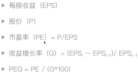
市盈率是什么
PEG策略说明
PEG选股
编码实现
市盈率有静态的和动态的两种,我们使用静态的pe_ratio,在valuation表中
收益增长率inc_net_profit_year_on_year,在indicator里面
# 导入函数库
from jqdata import *

# 初始化函数,设定基准等等
def initialize(context):
    set_benchmark('000300.XSHG') # 持有后不动
    set_option('use_real_price',True)
    set_order_cost(OrderCost(open_tax=0, close_tax=0.001, open_commission=0.0003,
    close_commission=0.0003, close_today_commission=0, min_commission=5), type='stock')

    # 选股范围
    g.security = get_index_stocks('000300.XSHG')
    g.q = query(valuation.code,valuation.pe_ratio,indicator.inc_net_profit_year_on_year).filter(valuation.code.in_(g.security))
    g.N = 20
    run_monthly(handle,1)

def handle(context):
    df = get_fundamentals(g.q)
    # 过滤负值的PEG
    df = df[(df['pe_ratio'] > 0) & (df['inc_net_profit_year_on_year'] > 0) ]
    # 计算peg
    df['peg'] = df['pe_ratio'] /df['inc_net_profit_year_on_year']/100
    df = df.sort_values('peg')
    to_hold = df['code'][:g.N].values
    print(to_hold)
    # 手上可能有一些股票,有的留着,没有的卖掉,添加新的
    for stock in context.portfolio.positions:
        # 手上的股票没在to_hold中,买掉
        if stock not in to_hold:
            order_target(stock,0)

    to_buy = [stock for stock in to_hold if stock not in context.portfolio.positions]

    if to_buy:
        cash_per_stock = context.portfolio.available_cash / len(to_buy)
        for per in to_buy:
            order_value(per,cash_per_stock)
动量策略和反转策略
编码实现
import jqdata
import math
import numpy as np
import pandas as pd
import datetime

def initialize(context):
    set_option('use_real_price', True)
    set_order_cost(OrderCost(open_tax=0, close_tax=0.001, open_commission=0.0003,
    close_commission=0.0003, close_today_commission=0, min_commission=5), type='stock')

    g.benchmark = '000300.XSHG'
    g.N = 10
    set_benchmark(g.benchmark)
    run_monthly(handle, 1)

def handle(context):
    stocks = get_index_stocks('000300.XSHG')
    # 这段时间的收盘价(attribu是选取一只股票多个时间的,history是选择多只股票)
    # 转置,相当于将股票代码放在了表头上
    df_close = history(30, field='close', security_list=list(stocks)).T
    # 增加ret列,表示收益率(最后一天的价格-第一天的价格)/ 第一天的价格
    df_close['ret'] = (df_close.iloc[:,-1]-df_close.iloc[:,0])/df_close.iloc[:,0]
    # ascending = False 表示降序,即为动量策略,总选最好的
    # ascending = True  反转策略
    sorted_stocks = df_close.sort_values('ret', ascending = False).index

    to_hold = sorted_stocks[:g.N]

    # 手上可能有一些股票,有的留着,没有的卖掉,添加新的
    for stock in context.portfolio.positions:
        # 手上的股票没在to_hold中,买掉
        if stock not in to_hold:
            order_target(stock,0)

    to_buy = [stock for stock in to_hold if stock not in context.portfolio.positions]

    if to_buy:
        cash_per_stock = context.portfolio.available_cash / len(to_buy)
        for per in to_buy:
            order_value(per,cash_per_stock)
最后得出结论,A股市场的反转策略优于动量策略
羊驼交易法则
编码实现
# 导入函数库
from jqdata import *

# 初始化函数,设定基准等等
def initialize(context):
    set_benchmark('000300.XSHG') # 持有后不动
    set_option('use_real_price',True)
    set_order_cost(OrderCost(open_tax=0, close_tax=0.001, open_commission=0.0003,
    close_commission=0.0003, close_today_commission=0, min_commission=5), type='stock')

    # 选股范围
    g.security = get_index_stocks('000300.XSHG')
    # 看多长时间的 收益率
    g.period = 30
    g.N = 10
    # 每次调整几只股票
    g.change = 1
    # 标志位,第一次购买的时候购买的是10只
    g.init = True
    run_monthly(handle,1)

def get_sorted_stocks(context,stocks):
    df_close = history(g.period, field='close', security_list=stocks).T
    # 增加ret列,表示收益率(最后一天的价格-第一天的价格)/ 第一天的价格
    df_close['ret'] = (df_close.iloc[:,-1]-df_close.iloc[:,0])/df_close.iloc[:,0]
    # ascending = False 表示降序,即为动量策略,总选最好的
    # ascending = True  反转策略
    sorted_stocks = df_close.sort_values('ret', ascending = False)
    return sorted_stocks.index.values


def handle(context):
    if g.init:
        stocks = get_sorted_stocks(context, g.security)[:g.N]
        cash = context.portfolio.available_cash * 0.9 / len(stocks)
        for stock in stocks:
            order_value(stock, cash)
        g.init = False
        return
    stocks = get_sorted_stocks(context, context.portfolio.positions.keys())

    for stock in stocks:
        if len(context.portfolio.positions) >= g.N:
            break
        if stock not in context.portfolio.positions:
            order_value(stock, context.portfolio.available_cash * 0.9)
简易回测框架开发
框架内容
- 上下文信息保存:context
- 获取数据:
- 下单函数:
- 用户接口:
- ...
来源:https://www.cnblogs.com/yxiaodao/p/10732824.html |



 發表於 2019-5-8 21:20:00